All posts by admin
Conda Environments
Computational Resources
Arina is composed of 2 subclusters: kalk2020 and kalk2017-katramila
As a whole, Arina features 147 nodes, which provide 196 multicore processors (CPUs) containing a total amount of 4396 cores.
Arina is equiped with two high performance file systems which provide a storage with total net capacity of 120 TB.
Within each subcluster the nodes are connected to each other via an Infiniband network characterized by high bandwith and low latency for intranode communications.
Subcluster kalk2020
The sublcluster kalk2020 features the following computing nodes:

In total, this set of nodes is composed of 45 computing nodes, which provide 90 multicore processors containing a total amount of 1800 cores.
This subcluster is endowed with a Parallel Cluster File System (BeeGFS) with a net capacity of 80 TB. Its storage is shared across the entire kalk2020 node compound.
The SLURM queue system is devoted to the management of the jobs submitted to kalk2020.
The intranode communication is speeded up thanks to an infiniband network with a transfer speed up to 100 Gb/s (EDR).
Subcluster kalk2017-katramila
This subcluster includes two sets of computing nodes, namely kalk2017 and katramila.
The kalk2017 node compound is composed of:

In total, it features 68 computing nodes, which provide 136 multicore processors containing a total amount of 1904 cores.
Each GPU Nvidia Tesla K40m features 2880 GPU cores and 12 GB of integrated GPU RAM.
The katramila node compound is composed of:

In total, it features 34 computing nodes, which provide 70 multicore processors containing a total amount of 692 cores.
Each GPU Nvidia Tesla K20m features 2496 GPU cores and 5 GB of integrated GPU RAM.
These two sets of computing nodes share a Parallel Cluster File System (Lustre) with a net capacity of 40 TB. Hence, Its storage is shared across the entire node compound of both kalk2017 and katramila.
The TORQUE/MAUI queue system is devoted to the management of the jobs submitted to kalk2017-katramila. Unless otherwise specified in the job submission, the queue system automatically sends jobs to either kalk2017 or katramila computing nodes upon node availability and requested resources.
The intranode communication is speeded up thanks to an infiniband network with a transfer speed up to 56 Gb/s (FDR).
Login
The access to the computational resources of Arina varies depending on the subcluster the user wants to log in and the Operating System (OS) of the workstation used for entering Arina.
IP addresses of the Arina subclusters
The IP address of the three current subclusters is:
agamede.lgp.ehu.es
kalk2020.lgp.ehu.es
kalk2017.lgp.ehu.es
katramila.lgp.ehu.es
for logging into agamede, kalk2020, kalk2017 and katramila, respectively.
How to log in Arina
The way the user can enter Arina strongly depends on the OS of the workstation/computer used for the connection to the cluster.
Unix/Linux, Mac OS
If the workstation employed for logging in Arina deploys either a Unix/linux or a Mac OS operating system, then the sole ssh protocol can be used.
Within the most common releases of these OSs, the ssh protocol is usually already activated. If not, look for instructions on how to activate it on the web.
In this case, follow these steps to establish a connection to kalk2020:
- Open a command line windows (by either clicking on the command line icon or typing command line in the OS browser bar)
- Type
ssh -X username@kalk2020.lgp.eus.es
where username is the user nickname in the cluster - Input the required user password
For entering kalk2017 and katramila, follow the same steps but change kalk2020.lgp.eus.es to either kalk2017.lgp.ehu.es or katramila.lgp.ehu.es, respectively.
The -X flag allows for the opening of Graphical User Interfaces (GUIs), namely program windows. In some cases, if you are working on a Mac OS workstation, you may need a third-party application to be able to launch GUIs: XQuartz. After its download and installation, make sure to launch it before trying to log in Arina.
Microsoft Windows
If the operating system of the device used for accessing Arina is Microsoft Windows, then a third-party software is necessary.
There are many pieces of software available on the web, such as MobaXterm, WinSCP, PuTTY, …
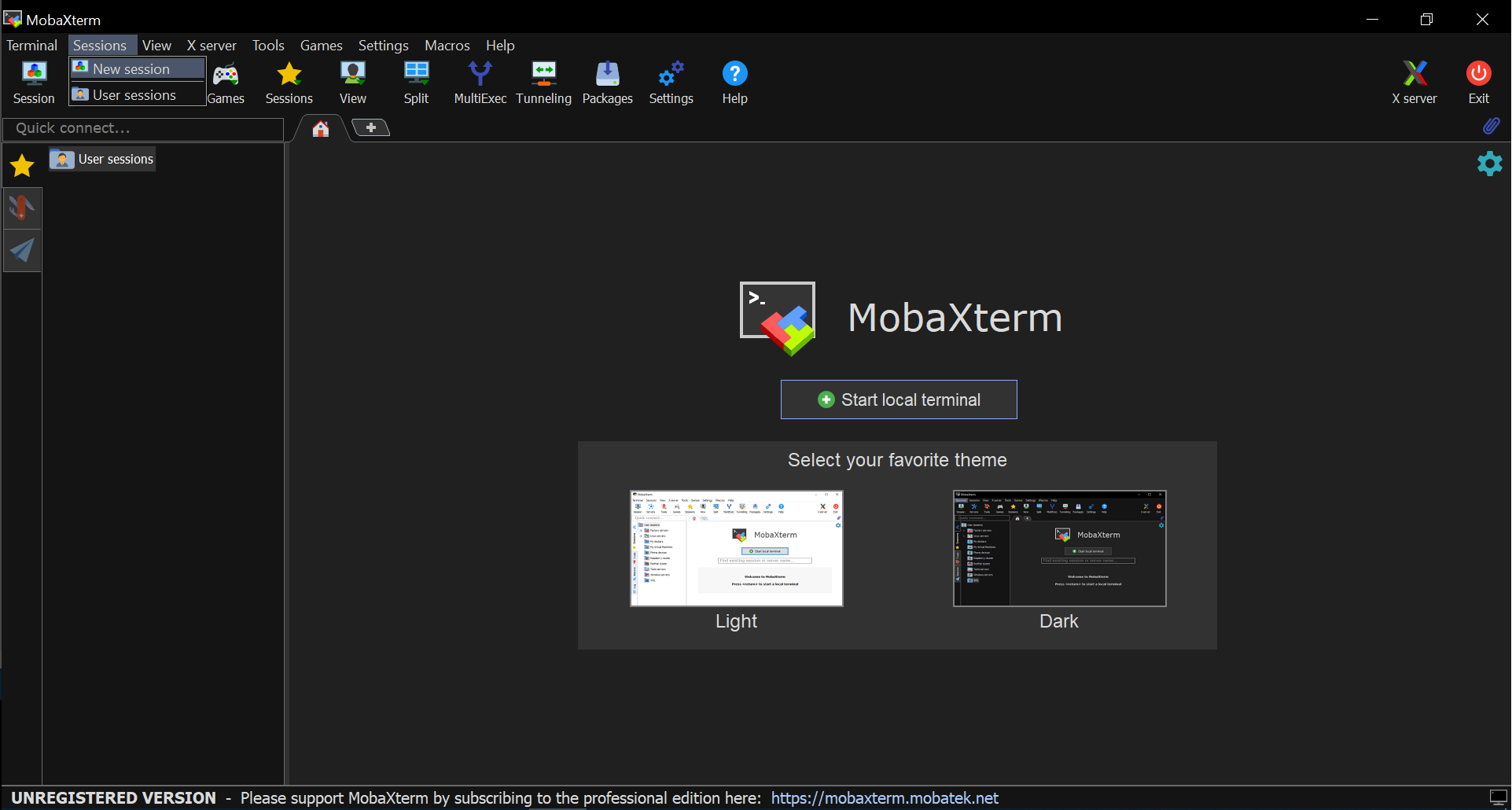
Here we show how to set up MobaXterm, which is the recommended one, but a similar configuration process could be followed for the rest of the mentioned software.
- Download MobaXterm from the web (if you prefer not to install the software, a portable version is also available): https://mobaxterm.mobatek.net/download.html
- Install the software and open it (or just open it if the portable version has been downloaded)
- Go to Sessions tab and select New session from the drop-down menu
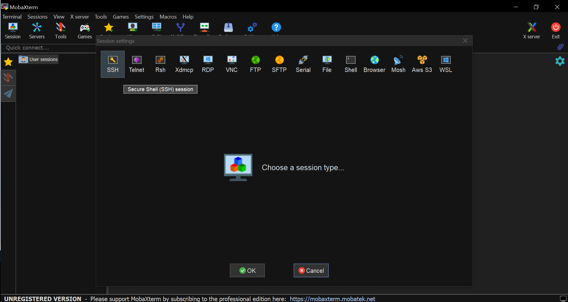
- Select the first icon (SSH) from the line-list on top of the pop-up window
- Fill in the Remote Host * gap with
kalk2020.lgp.ehu.es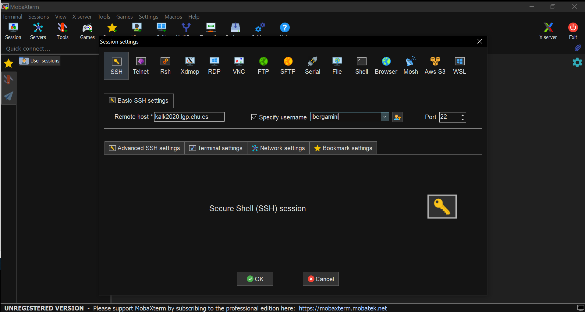
- Tick the Specify username box and insert the Arina nickname of the user in the gap next to it.
- Press the OK button.
- Input the required password.
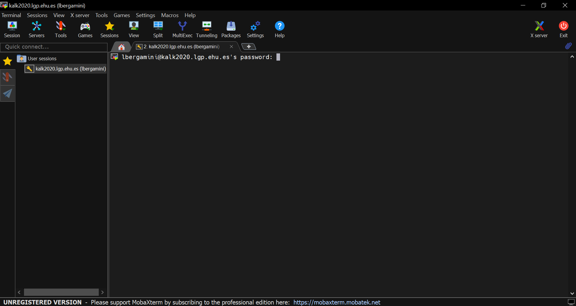
- A new session line will be created in the left panel below the User sessions folder. The session setup is now saved and can be loaded by just clicking twice on the session line in the left panel when you open MobaXterm. By clicking on it once, it is possible to rename it with an evocative name.
PSI4
General information
PSI4 is an open-source suite of ab initio quantum chemistry programs designed for efficient, high-accuracy simulations of a variety of molecular properties. It is very easy to use and has an optional Python interface.
How to Use
send_psi4
- To send PSI4 to the queue system use the send_psi4 utility. When executed,
shows the command syntax, which is summarized below: send_psi4 JOBNAME NODES PROCS_PER_NODE TIME [ MEM ] [``Other queue options'' ]
JOBNAME: Is the name of the input with extension. NODES: Number of nodes. PROCS: Number of processors. TIME: Time requested to the queue system, format hh:mm:ss. MEM: Optional. Memory in Gb ( It will used 1GB/core if not set). [``Other Torque Options'' ] Optional. There is the possibility to pass more variables to the queuing system.
See examples below. More information about this options
More information
VASP
General information
Vienna Ab-initio of Simulation Package
5.4.4 version of the DFT ab-initio program. It uses plane wave basis and pseudopotentials (ultrasoft and PAW-augmented wave method). VSTS tools has been included.
License is needed.
How to use
To usu VASP in parallel is enougth to execute:
/software/bin/vasp
[intlink id=”1353″ type=”post”]p4vasp[/intlink], [intlink id=”5514″ type=”post”]XCrySDen[/intlink] is installed.
v2xsf
Job monitorization
The convergence of a running job can be monitorized with:
remote_vi JOB_ID
that will open the OSZICAR and OUTCAR files in additon to plot the energy and energy variation. It is necessary to use ssh -X or to use X2GO to open the graphic windows.
More information
R, RCommander and RStudio
General information
R 3.3.3 is a freely available language and environment for statistical computing and graphics which provides a wide variety of statistical and graphical techniques: linear and nonlinear modelling, statistical tests, time series analysis, classification, clustering, etc. Please consult the R project homepage for further information.
RStudio an RCommander are a graphical front ends for R.
Installed packages
abind, ape, biomformat, cummeRbund, DCGL, DESeq2, DEXSeq, e1071, edgeR, FactoMineR, GEOquery, lavaan, metagenomeSeq, mnormt, optparse, psych, randomForest, Rcmdr, RColorBrewer, ReactomePA, RUVSeq, vegan, WGCNA, xlsx.
Please, ask if you need any more.
How to use it
To use R in the queue scripts execute:
/software/bin/R CMD BATCH R-input-file.R
to execute RStudio you must connect to Txinparta or Katramila with X2Go and execute
rstudio
to execute RCommander you must connect to Txinparta or Katramila with X2Go and execute R. Then inside R load
library(Rcmdr)
More information
SCIPION
General information
Scipion is an image processing framework to obtain 3D models of macromolecular complexes using Electron Microscopy. 2016 May version from Github.
How to use
To execute SCIPION use:
/software/bin/scipion
More information
AMBER
General information
14 version of AMBER (Assisted Model Building with Energy Refinement) and AMBER-tools15. Program with empiric potentials with molecular dynamics and energy minimization. Especially oriented to the simulation of biological systems.
How to use
The serial and parallel version have been compiled and can be found in the direktory
/software/bin/amber/
send_amber
To send jobs to the queue system you can use the send_amber command:
send_amber "Sander_options" Nodes Procs_Per_Node[property] Time [or Queue] [Mem]  ["Other_queue_options"]

Sander_options: the options you want to use in the calculation, inside quotes
Nodes: is the number of nodes
Procs: is the number of processors (you may uinclude the node type) per node.
Time: or Queue the walltime (in hh:mm:ss format) or the queue name of the calculation
Mem: the PBS memory (in gb)
[Mem] and ["Other_queue_options"] are optional
For “Other queue options” see examples below:
send_amber "sander.MPI -O -i in.md -c crd.md.23 -o file.out" job1 1 8 p_slow
send_amber "sander.MPI -O -i in.md -c crd.md.23 -o file.out" 2 8:xeon vfast 16 "-W depend=afterany:1234"
send_amber "sander.MPI -O -i in.md -c crd.md.23 -o file.out" 4 8 24:00:00 32 "-m be -M mi.email@ehu.es"
More information
Qbox
General Information
Version: 1.62.3
Qbox is a C++/MPI scalable parallel implementation of first-principles molecular dynamics (FPMD) based on the plane-wave, pseudopotential formalism. Qbox is designed for operation on large parallel computers.
How to use it:
To send qbox jobs to the queue we have created the send_qbox utility_
send_qbox JOBNAME NODES PROCS_PER_NODE[property] TIME
Executing send_box [Enter] more options will be shown. The program is installed in /software/qbox
More Information
On the Qbox Web page.
IDBA-UD
General information
IDBA-UD 1.1.1 is a iterative De Bruijn Graph De Novo Assembler for Short Reads Sequencing data with Highly Uneven Sequencing Depth. It is an extension of IDBA algorithm. IDBA-UD also iterates from small k to a large k. In each iteration, short and low-depth contigs are removed iteratively with cutoff threshold from low to high to reduce the errors in low-depth and high-depth regions. Paired-end reads are aligned to contigs and assembled locally to generate some missing k-mers in low-depth regions. With these technologies, IDBA-UD can iterate k value of de Bruijn graph to a very large value with less gaps and less branches to form long contigs in both low-depth and high-depth regions.
How to use
To send jobs to the queue you can use the command
send_idba-ud
which after a few questions configures the job.
Performance
IDBA-UD has a good performance and scaling up to 8 cores. Above we did not measure a improvement. In the benchmark the --mimk 40 --step 20 options has been used. When we have decreased the step the the scalling is worse. This trend can be also seen in the second table.
| 1 core as base | 2 cores as base | ||||
| Cores | Time (s) | Speed up | Performance (%) | Speed up | Performance (%) |
| 1 | 480 | 1 | 100 | ||
| 2 | 296 | 1.6 | 81 | 1.0 | 100 |
| 4 | 188 | 2.6 | 64 | 1.6 | 79 |
| 8 | 84 | 5.7 | 71 | 3.5 | 88 |
| 12 | 92 | 5.2 | 43 | 3.2 | 54 |
The second benchark has been done with a bigger file with 10 million bases and the --mink 20 --step 10 --min_support 2 options. We observe a regular behaviour than in the previous benchmark and how the panellization is good up to 4 cores.
| Cores | Time (s) | Speed up | Performance |
| 1 | 13050 | 1 | 100 |
| 2 | 6675 | 2.0 | 98 |
| 4 | 3849 | 3.4 | 85 |
| 8 | 3113 | 4.2 | 52 |
| 16 | 2337 | 5.6 | 35 |
| 20 | 2409 | 5.4 | 27 |
More information
IDBA-UD web page.
SPAdes
General information
SPAdes 3.6.0 – St. Petersburg genome assembler – is intended for both standard isolates and single-cell MDA bacteria assemblies. It works with Illumina or IonTorrent reads and is capable of providing hybrid assemblies using PacBio, Oxford Nanopore and Sanger reads. You can also provide additional contigs that will be used as long reads. Supports paired-end reads, mate-pairs and unpaired reads. SPAdes can take as input several paired-end and mate-pair libraries simultaneously. Note, that SPAdes was initially designed for small genomes. It was tested on single-cell and standard bacterial and fungal data sets.
How to use
To send jobs to the queue you can use the
send_spades
command that asks few questions to configure the job.
Performance
We have not measure any performance improvement or time reduction when using several cores in a standard calculation like:
spades.py -pe1-1 file1 -pe1-2 file2 -o outdir
We recommend to use 1 core, unless you know that you can use better performance with several cores.
More information
Web page of SPAdes.
MetAMOS
General information
MetAMOS represents a focused effort to create automated, reproducible, traceable assembly & analysis infused with current best practices and state-of-the-art methods. MetAMOS for input can start with next-generation sequencing reads or assemblies, and as output, produces: assembly reports, genomic scaffolds, open-reading frames, variant motifs, taxonomic or functional annotations, Krona charts and HTML report. 1.5rc3 version.
How to use
To send a job to the queue system there is the
send_metamos
command where you answer a few questions to set up the job. Take into account that MetAMOS use a lot of RAM memory, about 1 GB per million reads.
More information
MetAMOS web page.
QIIME
General information
QIIME (Quantitative Insights Into Microbial Ecology) is an open-source bioinformatics pipeline for performing microbiome analysis from raw DNA sequencing data. QIIME is designed to take users from raw sequencing data generated on the Illumina or other platforms through publication quality graphics and statistics. This includes demultiplexing and quality filtering, OTU picking, taxonomic assignment, and phylogenetic reconstruction, and diversity analyses and visualizations. QIIME has been applied to studies based on billions of sequences from tens of thousands of samples
How to use
To send QIIME jobs run the command
send_qiime
and answer the questions.
USEARCH
QIIME can use the [intlink id=”7744″ type=”post”]USEARCH[/intlink] pakage.
More information
[intlink id=”7700″ type=”post”]USEARCH[/intlink].
Mathematica
General Information
Mathematics program that includes symbolic and numeric computing, visualization and programing language. The 10.0 version is installed in Guinness, the 6.0 in the Itanium nodes. Katramila and the newest nodes has the 11.2 version.
Mathematica incluye paralelismo.
Ho to use Mathematica
In interactive mode
The graphical interface can be executed with
mathematica
and the Mathematica console with
math
Nota: If you have problems to visualize the fonts maybe you must install them in your local computer.
In the queue system
In the queue scripts use the line
/software/bin/math < input > output
whre input is the file with the Mathematica commands and output is the file where the output will be saved.
More information
R-3.2.0
General Information
R is ‘GNU S’, a freely available language and environment for statistical computing and graphics which provides a wide variety of statistical and graphical techniques: linear and nonlinear modelling, statistical tests, time series analysis, classification, clustering, etc. Please consult the R project homepage for further information.
Installed Packages
lavaan, mnormt, psych, Rcmdr, abind, e1071, xlsx, biocLite(),FactoMineR
Please ask if you need any more.
How to use it
To use R-3.2 execute:
/software/R-3.2.0/bin/R CMD BATCH input.R
More Information:
USEARCH
General information
USEARCH is a unique sequence analysis tool that offers search and clustering algorithms that are often orders of magnitude faster than BLAST. We have the free 32 bits version that can not be distributed to third parties and has a 4 GB of RAM limitation.
How to use
To use USEARCH execute
/software/bin/usearch
for example
/software/bin/usearch -cluster_otus data.fa -otus otus.fa -uparseout out.up -relabel OTU_ -sizein -sizeout
USEARCH is only available in the xeon20 type nodes.
QIIME
USEARCH can be use under [intlink id=”7758″ type=”post”]QIIME[/intlink].
More information
[intlink id=”7686″ type=”post”]QIIME[/intlink].
SAMtools, BCFtools and HTSlib 1.2
General Information
Samtools is a suite of programs for interacting with high-throughput sequencing data. It consists of three separate repositories:
Samtools
Reading/writing/editing/indexing/viewing SAM/BAM/CRAM format
BCFtools
Reading/writing BCF2/VCF/gVCF files and calling/filtering/summarising SNP and short indel sequence variants
HTSlib
A C library for reading/writing high-throughput sequencing data
Samtools and BCFtools both use HTSlib internally, but these source packages contain their own copies of htslib so they can be built independently.
How to use It
They are installed in /software/samtools-1.2/, /software/bcftools-1.2/ and /software/htslib-1.2.1 respectibely.
Something like this should be added in the PBS script.
export PATH=/software/samtools-1.2/bin:/software/bcftools-1.2/bin:$PATH
export LD_LIBRARY_PATH=/software/htslib-1.2.1/lib:$LD_LIBRARY_PATH
More Information
GSL
GNU Scientific Libraries for randon number generators, linear algebra, FFT, special functions, etc
To know how to use the
gsl-config
More information at GSL homepage.
How to submit siesta jobs
How to submit siesta jobs
There are three ways:
- Using the
send_siestacommand. - Using
qsubin interactive way. - With a scritp for the
qsubcommand.
send_siesta
We have written the send_siesta command to submit Siesta jobs. Execute send_siesta and its usage is shownArina. In the following lines we describe it sintax-
send_siesta JOBNAME NODES PROCS_PER_NODE[property] TIME MEM ["Other queue options"]
JOBNAME: Input file without extension.
NODES: Number of nodes to be used.
PROCS_PER_NODE: Cores per node.
TIME: Walltime in hh:mm:ss format.
MEM: Memoria Gb unitatetan.
["Other queue options"]Other instructions to the queue system inside quotes.
Examples
To submit the job1.fdf input in one itaniumb node and for cores:
send_siesta job1 1 4:itaniumb 04:00:00 1
To submit the job2.fdf input to 2 nodes and for cores in each node, 192 hours and 8gb RAM memory. In adition, the job will start after the job with 1234 identifier finish:
send_siesta job2 2 4 192:00:00 8 ``-W depend=afterany:1234''
To submit the job2.fdf input file in 4 nodes and 8 cores per node, 200 hours, eta 15gb RAM. In addition send an email when the jobs starts and finish:
send_siesta job2 4 8 200:00:00 15 ``-m be -M nire.emaila@ehu.es''
The send_siesta command will use the local /scratch directory or the global file system /gscratch depending on the number of nodes used.
Interactive qsub
Exekute
qsub
without arguments and answer the question.
Regular qsub
Build a script for qsub,[intlink id=”237″ type=”post”] here there are examples[/intlink], and to execute Siesta use the following line
/software/bin/siesta/siesta_mpi < input.fdf > log.out
Job monitoring
- If you used
send_siesta
- or interactive
qsub
- to submit a job you can monitor it with the following commands:
- remote_vi
- It will open the *.out file with gvim.
- remote_xmakemol
- xmakemol will be used to open the *.ANI file.
- remote_qmde
- xmgrace will be used to plot energia vs. time in molecular dynamics simulations.
Examples to monitor the job with 3465 identifier:
remote_vi 3465
remote_xmakemol 3465
remote_qmde 3465
Siesta
General information
Spanish Initiative for Electronic Simulation with Thousands Atoms. DFT based simulation program for solids and molecules. It can be used for molecular dynamics and relaxations. It uses localized orbitals that allow to make calculations with large number of atoms. The academic license is freely distributed but it is necessary to ask for a license. The 3.0rc1 version is installed in the x87_64 nodes and the 2.0.1 in the Itanium nodes.
How to send siesta
[intlink id=”7224″ type=”post”]Follow this link[/intlink].
More information
Trinity
General information
2.1.1 release. Trinity, represents a novel method for the efficient and robust de novo reconstruction of transcriptomes from RNA-seq data. Trinity combines three independent software modules: Inchworm, Chrysalis, and Butterfly, applied sequentially to process large volumes of RNA-seq reads. Trinity partitions the sequence data into many individual de Bruijn graphs, each representing the transcriptional complexity at at a given gene or locus, and then processes each graph independently to extract full-length splicing isoforms and to tease apart transcripts derived from paralogous genes. Briefly, the process works like so:
- Inchworm assembles the RNA-seq data into the unique sequences of transcripts, often generating full-length transcripts for a dominant isoform, but then reports just the unique portions of alternatively spliced transcripts.
- Chrysalis clusters the Inchworm contigs into clusters and constructs complete de Bruijn graphs for each cluster. Each cluster represents the full transcriptonal complexity for a given gene (or sets of genes that share sequences in common). Chrysalis then partitions the full read set among these disjoint graphs.
- Butterfly then processes the individual graphs in parallel, tracing the paths that reads and pairs of reads take within the graph, ultimately reporting full-length transcripts for alternatively spliced isoforms, and teasing apart transcripts that corresponds to paralogous genes.
How to use
You can use the
send_trinity
command to submit jobs to the queue system. After answering few questions a script will be created and submitted to the queue system. For advanced users it can be used to generate a sample script.
Performance
Trinity can be run in parallel but it is not very efficient above 4 cores with low performance, as can be seen in the the table. Trinity consumes high amounts of RAM.
| Cores | 1 | 4 | 8 | 12 |
| Time | 5189 | 2116 | 1754 | 1852 |
| Speddup | 1 | 2.45 | 2.96 | 2.80 |
| Efficiency (%) | 100 | 61 | 37 | 23 |
More information
PHENIX
General information
Versión dev-2229 (higher than 1.10) of PHENIX (Python-based Hierarchical ENvironment for Integrated Xtallography). PHENIX is a software suite for the automated determination of macromolecular structures using X-ray crystallography and other methods. It is ready to use with [intlink id=”1969″ type=”post”]AMBER[/intlink].
How to use
To execute the graphical interface in Guinness execute the command:
phenix &
To execute PHENIX in the queue system scripts the PHENIX working environment must be loaded first with the source command. Execute for example:
phenix.xtriage my_data.sca [options]
More information
PHENIX web page.
Online documentation.
Documentation in pdf.
FFTW libraries
Fastest Fourier Transform in the West to make all type of Fourier transforms.
The 3.3.3 version is installed in /software/fftw. Several types have been compiled (threads, simple precission,etc)
To link them use
-L/software/fftw -lfftw3
If you have doubts ask the technicians.
More information in the web page FFTW.
Abinit
General Information
ABINIT is a package whose main program allows one to find the total energy, charge density and electronic structure of systems made of electrons and nuclei (molecules and periodic solids) within Density Functional Theory (DFT), using pseudopotentials and a planewave or wavelet basis. ABINIT also includes options to optimize the geometry according to the DFT forces and stresses, or to perform molecular dynamics simulations using these forces, or to generate dynamical matrices, Born effective charges, and dielectric tensors, based on Density-Functional Perturbation Theory, and many more properties. Excited states can be computed within the Many-Body Perturbation Theory (the GW approximation and the Bethe-Salpeter equation), and Time-Dependent Density Functional Theory (for molecules). In addition to the main ABINIT code, different utility programs are provided. netcdf, bigdft, wannier90, etsf_io, libxc, etc. plugins are included. 7.0.4 version is installed.
How to send Abinit
The programs are in /software/bin/abinit. For instance, to execute abinit in the queue system scripts use
/software/bin/abinit/abinit < input.files > out.log
Depending on the number of cores asked to the queue system it will execute in parallel. The jobs can be also submitted with the [intlink id=”233″ type=”post”]interactive qsub[/intlink] command.
There are other utilities like aim, anaddb, band2eps, conducti, cut3d, lwf, macroave, mrgddb, mrggkk, newsp, optic, etc.
Benchmark
We have made a small benchmark with the 6.12.3 version.
| System | 1 cores | 4 cores | 8 cores |
| Xeon12 | 7218 | 2129 | 1045 |
| Xeon8 | 7275 | 1918 | 1165 |
| Itanium | 8018 | 2082 | 1491 |
| Opteron | 17162 | 4877 | 2802 |
We observe that Abinit works fine in itanium and xeon nodes while in opteron nodes is slower.
More information
Internal User Rates
General Information
The internal rate applies to researchers and centers of the UPV / EHU. Includes service and applications. The rates will be valid from 15-09-2021 to 14-09-2022.
CPU usage charges
The fee for a research group will be 0.005 € / hour and core.
Storage Rates
Every user has a 3 gb storage quota taht will not be charged. Having more data in Arina will be charged as follows:
| CPU usage Range | Storage Fee | ||
| (in days per year) | (€/Gb) per month | ||
| 2500< | cpu | 0.1 | |
| 100< | cpu | <2500 | 0.5 |
| 1< | cpu | <100 | 1.0 |
| 0< | cpu | <1 | 1.5 |
CPU usage charges until 08-31-2019
The fee for a research group will be:
- 0.011 € / hour and core until the group reaches the use of 18.939,39 days of calculation (corresponding to 5.000 €).
- Once this consumption is reached , the rest of the computing time will be charged at 0.003€ / hour and core.
ABySS
General Information
1.3.2 version of ABySS (Assembly By Short Sequences). ABySS is a de novo, parallel, paired-end sequence assembler that is designed for short reads. ABySS can be executed in parallel.
See also the installed [intlink id=”6043″ type=”post”]velvet[/intlink] and comparing both we have published article.
How to use
The executables can be found in /software/abyss/bin. To run abyss in a script type in it:
/software/abyss/bin/abyss-pe [abyss-pe options]
Performance
See also the installed [intlink id=”6043″ type=”post”]velvet[/intlink] and comparing both we have published article.
Parallelization
Some benchmarks has been performed with ABySS. They have been performed using file from an Illumina HiSeq2000 NGS with 100 bp per sequence. In the table 1 we can see an example about how ABySS scales as a function of the number of cores. As we can see ABySS scales very up to 8 cores. The results is valid unless for more than 10e6 sequences.
| cores | 2 | 4 | 8 | 12 | 24 |
| Time (s) | 47798 | 27852 | 16874 | 14591 | 18633 |
| Aceleration | 1 | 1.7 | 2.8 | 3.3 | 2.6 |
| Performance(%) | 100 | 86 | 71 | 55 | 21 |
Execution time
We have analized as well the execution time as a function of the size of the data. In the table 2 we observe how from 1 million to 10 millions of sequences the execution time increases by 10 as well. From 10 to 100 millions of sequences the time increases a little more, between 10 t0 20. Therefore, the behavior is more or less lineal.
| sequences | 10e6 | 10e7 | 10e8 |
| Time in 2 cores (s) | 247 | 2620 | 47798 |
| Time in 4 cores (s) | 134 | 1437 | 27852 |
| Time in 8 cores (s) | 103 | 923 | 16874 |
RAM memory
In these kind of programs more important than the execution time, which is reasonable, is the RAM memory usage, which can limit the calculation type. In the table 3 we observe how the RAM increases as a function of the number of sequences. We also show the logarithms of the measured values which has been used for a lineal regression. The jobs has been performed in 12 cores.
| sequences | 10e6 | 5*10e6 | 10e7 | 5*10e7 | 10e8 |
| RAM (GB) | 4.0 | 7.6 | 11 | 29 | 44 |
| log(sequences) | 6 | 6.7 | 7 | 7.7 | 8 |
| log(RAM) | 0.60 | 0.88 | 1.03 | 1.46 | 1.65 |
From the values of the table we obtain a fitting of the RAM in GB as a function of the number of sequences (s) to the equation
log(RAM)=0.53*log(s)-2.65
o equivalently
RAM=(s^0.53)/447
Conclusion
The memory usage is smaller than in other assemblers like [intlink id=”6043″ type=”post”]Velvet[/intlink], see as well the report Velvet performance in the machines of the Computing Service of the UPV/EHU and comparing both we have published article. In addition, the parallelization with MPI of ABySS allows to aggregate the RAM memory of several nodes to perform larger calculations.
More information
ABySS web page.
[intlink id=”6043″ type=”post”]Velvet[/intlink] assembler.
Velvet performance in the machines of the Computing Service of the UPV/EHU report.
Velvet and ABySS performance in the machines of the Computing Service of the UPV/EHU, post in the hpc blog.
abyss-peClean reads
General information
0.2.2 Version. clean_reads cleans NGS (Sanger, 454, Illumina and solid) reads. It can trim:
- bad quality regions
- adaptors
- vectors
- regular expresssions
It also filters out the reads that do not meet a minimum quality criteria based on the sequence length and the mean quality. It can run in parallel.
Ho to use
To submit clean_reads jobs to the queue system execute the command
send_clean_reads
It will ask few questions to build the script and submit it to the queue.
Performance
clean_reads can be executed in parallel and scales well up to 8 cores. For 12 cores the performance is very poor. In the table 1 we show the results of the benchmark. They have been executed in a 12 cores node with E5645 Xeon processors.
| cores | 1 | 4 | 8 | 12 |
| Time (s) | 1600 | 422 | 246 | 238 |
| Speedup | 1 | 3.8 | 6.5 | 6.7 |
| Performance (%) | 100 | 95 | 81 | 56 |
The used command has been
clean_reads -i in.fastq -o out.fastq -p illumina -f fastq -g fastq -a a.fna -d UniVec -n 20 --qual_threshold=20 --only_3_end False -m 60 -t 12
More information
Velvet
General information
1.2.03 version. Velvet is a set of algorithms manipulating de Bruijn graphs for genomic and de novo transcriptomic Sequence assembly. It was designed for short read sequencing technologies, such as Solexa or 454 Sequencing and was developed by Daniel Zerbino and Ewan Birney at the European Bioinformatics Institute. The tool takes in short read sequences, removes errors then produces high quality unique contigs. It then uses paired-end read and long read information, when available, to retrieve the repeated areas between contigs.
See also the installed [intlink id=”6200″ type=”post”]ABySS[/intlink] and comparing both we have published article.
How to use
To run velveth or velvetg add in your scripts for the Torque queue system the corresponding command:
/software/bin/velvet/velveth [velvet options]
/software/bin/velvet/velvetg [velvet option]
Performance
Velvet has been compiled with parallel support througth OpenMP. We have measured the perfomance and the results are available in the report about the Velvet performance in the machines of the Computing Service of the UPV/EHU. Velvet uses huge amount of RAM for large calculations and we have measured it. In the report some simple formulas are obtained to predict the use of RAM for their input files, so the researches can know the needed RAM before start the calculations and in this way can plan their research.
See also the installed [intlink id=”6200″ type=”post”]ABySS[/intlink] and comparing both we have published article.
More information
Velvet web page.
Velvet performance in the machines of the Computing Service of the UPV/EHU report.
Velvet and ABySS performance in the machines of the Computing Service of the UPV/EHU, post in the hpc blog.
BLAST
General Information
2.2.24 version of BLAST de NCBI. Due to performance reasons it has not been installed in Itanium nodes.
Data bases
The Service has installed several data bases, contact the technicians to use them or install new ones.
How to use
To submit jobs to the queue system we strongly recomend to use the command
send_blast
it will make some questions to prepare the job
Performance and gpuBLAST
We have compared BLAST with mpiBLAST and gpuBLAST, the result of the bechmarks are in the blog of Service. [intlink id=”1495″ type=”post” target=”_blank”]mpiBLAST[/intlink] is installed in the Service.
More information
[intlink id=”1493″ type=”post”]Blast2GO[/intlink] y [intlink id=”1495″ type=”post” target=”_blank”]mpiBLAST[/intlink] is also installed.
Genepop
General information
4.1 version.
Genepop is a population genetics software package, which has options for the following analysis: Hardy Weinberg equilibrium, Linkage Disequilibrium, Population Differentiation, Effective number of migrants, Fst or other correlations.
How to use
To execute Genepop in the queue system you must include in the script of the queue system:
/software/bin/Genepop < input_file
where input_file has the options for Genepop, i.e., the answer to Genepop when it runs in interactive mode. We recommend to use [intlink id=”233″ type=”post”]qsub in interactive mode[/intlink] to submit the jobs
More information
CLUMPP
General information
1.1.3 version. CLUMPP is a program that deals with label switching and multimodality problems in population-genetic cluster analyses. CLUMPP permutes the clusters output by independent runs of clustering programs such as [intlink id=”5875″ type=”post”]structure[/intlink], so that they match up as closely as possible. The user has the option of choosing one of three algorithms for aligning replicates, with a tradeoff of speed and similarity to the optimal alignment.
How to use
To execute CLUMPP in the queue system you must include in the script of the queue system:
/software/bin/CLUMPP
with the corresponding options of structure. We recommend to use [intlink id=”233″ type=”post”]qsub in interactive mode[/intlink] to submit the jobs
More information
Structure
General information
2.33 version.
The program structure is a free software package for using multi-locus genotype data to investigate population structure. Its uses include inferring the presence of distinct populations, assigning individuals to populations, studying hybrid zones, identifying migrants and admixed individuals, and estimating population allele frequencies in situations where many individuals are migrants or admixed. It can be applied to most of the commonly-used genetic markers, including SNPS, microsatellites, RFLPs and AFLPs.
How to use
To execute the graphical user interface execute in Péndulo, Maiz or Guinness
structure
To execute graphical applications read [intlink id=”48″ type=”post”]how to connect to Arina[/intlink].
To execute structure in the queue system you must include in the script of the queue system:
/software/bin/structure
with the corresponding options of structure. We recommend to use [intlink id=”233″ type=”post”]qsub in interactive mode[/intlink] to submit the jobs
More information
MCCCS Towhee 7.0.2
Towhee is a Monte Carlo molecular simulation code originally designed for the prediction of fluid phase equilibria using atom-based force fields and the Gibbs ensemble with particular attention paid to algorithms addressing molecule conformation sampling. The code has subsequently been extended to several ensembles, many different force fields, and solid (or at least porous) phases.
General Information
Towhee serves as a useful tool for the molecular simulation community and allows science to move forward more quickly by eliminating the need for individual research groups to rewrite routines that already exist and instead allows them to focus on algorithm advancement, force field development, and application to interesting systems.
Towhee may use different type of ensembles and Monte Carlo moves implemented into Towhee and can alos used different force fields included with the distribution. (See here for more information )
How to Use
send_towhee
- To send Towhee to the queue system use the send_gulp utility. When executed,
shows the command syntax, which is summarized below: - send_towhee JOBNAME NODES PROCS_PER_NODE TIME [ MEM ] [``Other queue options'' ]
| JOBNAME: | Is the name of the Output. |
| NODES: | Number of nodes. |
| PROCS: | Number of processors. |
| TIME: | Time requested to the queue system, format hh:mm:ss. |
| MEM: | Optional. Memory in Gb ( It will used 1GB/core if not set). |
| [``Other Torque Options'' ] | Optional. There is the possibility to pass more variables to the queuing system. See examples below. More information about this options |
Examples
We send a Towhee job1 to 1 node, 4 processors on that node, with a requested time of 4 hours . The results will be in the OUT file.
send_towhee OUT 1 4 04:00:00
We send job2 to 2 compuation nodes, 8 processors on each node, with a requested time of 192 hours, 8 GB of RAM and to start running after work 1234.arinab is finished:
send_towhee OUT 2 8 192:00:00 8 ``-W depend=afterany:1234'
We send the input job3 to 4 nodes and 4 processors on each node, with arequested time of 200:00:00 hours, 2 GB of RAM and we request to be send an email at the beginning and end of the calculation to the direction specified.
send_towhee OUT 4 4 200:00:00 2 ``-m be -M mi.email@ehu.es''
send_towhee command copies the contents of the directory from which the job is sent to /scratch or / gscratch, if we use 2 or more nodes. And there is where the calculation is done.
Jobs Monitoring
To facilitate monitoring and/or control of the Towhee calculations, you can use remote_vi
remote_vi JOBID
It show us the *.out file (only if it was sent using send_towhee).
More information
Gulp 4.0
General Information
GULP is a program for performing a variety of types of simulation on materials using boundary conditions of 0-D (molecules and clusters), 1-D (polymers), 2-D (surfaces, slabs and grain boundaries), or 3-D (periodic solids). The focus of the code is on analytical solutions, through the use of lattice dynamics, where possible, rather than on molecular dynamics. A variety of force fields can be used within GULP spanning the shell model for ionic materials, molecular mechanics for organic systems, the embedded atom model for metals and the reactive REBO potential for hydrocarbons. Analytic derivatives are included up to at least second order for most force fields, and to third order for many.
How to Use
First, before you use it, be aware of its usage conditions.
send_gulp
- To send GULP to the queue system use the send_gulp utility. When executed,
shows the command syntax, which is summarized below: - send_gulp JOBNAME NODES PROCS_PER_NODE TIME [ MEM ] [``Other queue options'' ]
| JOBNAME: | Is the name of the input with extension. |
| NODES: | Number of nodes. |
| PROCS: | Number of processors. |
| TIME: | Time requested to the queue system, format hh:mm:ss. |
| MEM: | Optional. Memory in Gb ( It will used 1GB/core if not set). |
| [``Other Torque Options'' ] | Optional. There is the possibility to pass more variables to the queuing system. See examples below. More information about this options |
Examples
We send the GULP input job1 to 1 node, 4 processors on that node, with a requested time of 4 hours :
send_gulp job1.gin 1 4 04:00:00
We send job2 to 2 compuation nodes, 8 processors on each node, with a requested time of 192 hours, 8 GB of RAM and to start running after work 1234.arinab is finished:
send_gulp job2.gin 2 8 192:00:00 8 ``-W depend=afterany:1234'
We send the input job3 to 4 nodes and 4 processors on each node, with arequested time of 200:00:00 hours, 2 GB of RAM and we request to be send an email at the beginning and end of the calculation to the direction specified.
send_gulp job.gin 4 4 200:00:00 2 ``-m be -M mi.email@ehu.es''
send_gulp command copies the contents of the directory from which the job is sent to /scratch or / gscratch, if we use 2 or more nodes. And there is where the calculation is done.
Jobs Monitoring
To facilitate monitoring and/or control of the GULP calculations, you can use remote_vi
remote_vi JOBID
It show us the *.out file (only if it was sent using send_lmp).
More information
LAMMPS
LAMMPS (“Large-scale Atomic/Molecular Massively Parallel Simulator”) is a molecular dynamics program from Sandia National Laboratories. LAMMPS makes use of MPI for parallel communication and is a free open-source code, distributed under the terms of the GNU General Public License.
LAMMPS was originally developed under a Cooperative Research and Development Agreement (CRADA) between two laboratories from United States Department of Energy and three other laboratories from private sector firms. It is currently maintained and distributed by researchers at the Sandia National Laboratories. (Taken from Wikipedia). Jun-05-2019 version.
General Information
LAMMPS is a classical molecular dynamics code that models an ensemble of particles in a liquid, solid, or gaseous state. It can model atomic, polymeric, biological, metallic, granular, and coarse-grained systems using a variety of force fields and boundary conditions.
In the most general sense, LAMMPS integrates Newton’s equations of motion for collections of atoms, molecules, or macroscopic particles that interact via short- or long-range forces with a variety of initial and/or boundary conditions. For computational efficiency LAMMPS uses neighbor lists to keep track of nearby particles. The lists are optimized for systems with particles that are repulsive at short distances, so that the local density of particles never becomes too large. On parallel machines, LAMMPS uses spatial-decomposition techniques to partition the simulation domain into small 3d sub-domains, one of which is assigned to each processor. Processors communicate and store “ghost” atom information for atoms that border their sub-domain. LAMMPS is most efficient (in a parallel sense) for systems whose particles fill a 3d rectangular box with roughly uniform density. Papers with technical details of the algorithms used in LAMMPS are listed in this section.
How to Use
send_lmp
- To send LAMMPS to the queue system use the send_lmp utility. When executed,
shows the command syntax, which is summarized below: send_lmp JOBNAME NODES PROCS_PER_NODE TIME [ MEM ] [``Other queue options'' ]
JOBNAME: Is the name of the input with extension. NODES: Number of nodes. PROCS: Number of processors. TIME: Time requested to the queue system, format hh:mm:ss. MEM: Optional. Memory in Gb ( It will used 1GB/core if not set). [``Other Torque Options'' ] Optional. There is the possibility to pass more variables to the queuing system.
See examples below. More information about this options
Examples
We send the lammps input job1 to 1 node, 4 processors on that node, with a requested time of 4 hours:
send_lmp job1.in 1 4 04:00:00
We send job2 to 2 compuation nodes, 8 processors on each node, with a requested time of 192 hours, 8 GB of RAM and to start running after work 1234.arinab is finished:
send_lmp job2.inp 2 8 192:00:00 8 ``-W depend=afterany:1234'
We send the input job3 to 4 nodes and 4 processors on each node, with arequested time of 200:00:00 hours, 2 GB of RAM and we request to be send an email at the beginning and end of the calculation to the direction specified.
send_lmp job.tpr 4 4 200:00:00 2 ``-m be -M mi.email@ehu.es''
send_lmp command copies the contents of the directory from which the job is sent to /scratch or / gscratch, if we use 2 or more nodes. And there is where the calculation is done.
Jobs Monitoring
To facilitate monitoring and/or control of the LAMMPS calculations, you can use remote_vi
remote_vi JOBID
It show us the *.out file (only if it was sent using send_lmp).
More information
XCrySDen
General information
XCrySDen is a crystalline and molecular structure visualisation program, which aims at display of isosurfaces and contours, which can be superimposed on crystalline structures and interactively rotated and manipulated.
How to use
To use XCrySDen execute:
xcrysden
More information
GRETL
General information
Gretl (Gnu Regression, Econometrics and Time-series Library) is a software for econometric analysis. 1.9.6 version is installed.
Charateristics
- Incluye una gran variedad de estimadores: mínimos cuadrados, máxima verosimilitud, GMM; de una sola ecuación y de sistemas de ecuaciones
- Métodos de series temporales: ARMA, GARCH, VARs y VECMs, contrastes de raíces unitarias y de cointegración, etc.
- Variables dependientes limitadas: logit, probit, tobit, regresión por intervalos, modelos para datos de conteo y de duración, etc.
- Los resultados de los modelos se pueden guardar como ficheros LaTeX, en formato tabular y/o de ecuación.
- Incluye un lenguaje de programación vía ‘scripts’ (guiones de instrucciones): las órdenes se pueden introducir por medio de los menús o por medio de guiones.
- Estructura de bucles de instrucciones para simulaciones de Monte Carlo y procedimientos de estimación iterativos.
- Controlador gráfico mediante menús, para el ajuste fino de los gráficos Gnuplot.
- Enlace a GNU R, GNU Octave y Ox para análisis más sofisticados de los datos.
How to use
In order to use Gretl execute
/software/bin/gretlcli
More information
HMPP
General information
Based on C and FORTRAN directives, HMPP Workbench version 2.5.2 offers a high level abstraction for GPGPUs. HMPP compiler integrates powerful data-parallel backends for NVIDIA CUDA and OpenCL. The HMPP runtime ensures application deployment on multi-GPU systems.
How to use
In order to execute the compiler use
hmpp
for example, to compile the test.c program by using the gcc compiler use
hmpp gcc test.c -o test
More information
Gaussview
5.0.9 version of Gaussview, GUI to create and analyze [intlink id=”12″ type=”post”]Gaussian[/intlink] jobs. In order to use it, execute:
gv
We strongly recommend to use it through an NX-client in Guinness. You can find information about how to configure NX-client correctly in the following step by step guide.
CPLEX
General information
IBM ILOG CPLEX Optimizer’s mathematical optimization technology enables smarter decision-making for efficient resource utilization. CPLEX provides robust algorithms for demanding problems: IBM ILOG CPLEX Optimizer has solved problems with millions of constraints and variables. 12.6.3 version.
Features
- Automatic and dynamic algorithm parameter control
IBM ILOG CPLEX Optimizer automatically determines “smart” settings for a wide range of algorithm parameters, usually resulting in optimal linear programming solution performance. However, for a more hands-on approach, dozens of parameters may be manually adjusted, including algorithmic strategy controls, output information controls, optimization duration limits, and numerical tolerances. - Fast, automatic restarts from an advanced basis
Large problems can be modified, and then solved again in a fraction of the original solution time. - A variety of problem modification options, such as:
– The ability to add and delete variables
– The ability to add and delete constraints
– The ability to modify objective, right-hand side, bound and matrix coefficients
– The ability to change constraint types - A wide variety of input/output options, such as:
– Problem files: read/write MPS files, IBM ILOG CPLEX Optimizer LP files, MPS basis and revise files, binary problem/basis files
– Log files: session information and various solution reports
– Solution files: ASCII and binary solution files
– IBM ILOG CPLEX Optimizer messages: Each message type (such as RESULTS, WARNINGS or ERRORS) can be directed to specified files, or completely suppressed. - Post solution information and analysis, including:
– Objective function value
– Solution variable and slack values
– Constraint dual values (shadow prices)
– Variable reduced costs
– Right-hand side, objective function, and bound sensitivity ranges
– Basic variables and constraints
– Solution infeasibilities (if any exist)
– Iteration/node count, solution time, process data
– Infeasibility (IIS) finder for diagnosing problem infeasibilities
– Feasibility optimizer for automatic correction of infeasible models
How to use
To use CPLEX execute:
/software/bin/cplex/cplex
Benchmark
There is a small benchmark usingCOIN-OR, see [intlink id=”5224″ type=”post”]COIN-OR web page[/intlink].
More information
COIN-OR
General information
1.7.5 version. The Computational Infrastructure for Operations Research (COIN-OR**, or simply COIN) project is an initiative to spur the development of open-source software for the operations research community. It has been konpiled using [intlink id=”5240″ type=”post”]CPLEX[/intlink].
How to use
The blis, cbc, clp, OSSolverService and symphony executables are installed in /software/bin/CoinAll. To use, for example, clp execute in the torque scripts:
/software/bin/CoinAll/clp
More information
DL_POLY
General information
4.02 version of the MD program for macromolecules, polymers, ionic systems, solutions and other molecular systems. Developed at the Daresbury Laboratory. In Pendulo the 2.2 version remains. There is already the DL_POLY_CLASSIC version which currently is not been developed.
How to submit to the queue
The program is installed in all the architectures, Arina and Pendulo (DL_POLY 2.2). To execute it include in the scripts:
/software/bin/DL_POLY/DL_POLY.Z
The program will exekute in GPGPUs if it starts in these kind of nodes. Besides, they can be selected by using the gpu label within [intlink id=”244″ type=”post”]the queue system[/intlink].
The GUI is also installed. To execute it use:
/software/bin/DL_POLY/gui
Some utilities has been installed in the /software/bin/DL_POLY/ directory.
Benchmark
We show a small benchmarks performed with dl_ploly_4.02. We stady the parallelization as well as the performance of the GPGPUs.
| System | 1 cores | 4 cores | 8 cores | 16 cores | 32 cores | 64 cores |
| Itanium 1.6 GHz | 1500 | 419 | 248 | 149 | 92 | 61 |
| Opteron | 1230 | 503 | 264 | 166 | 74 | |
| Xeon 2.27 GHz | 807 | 227 | 126 | 67 | 37 | 25 |
We show in the firs benchamrk that DL_POLY scales very well and that the xeon nodes are the fastest ones, so we recomend them for large jobs.
| System | 1 cores | 2 cores | 4 cores | 8 cores | 16 cores | 32 cores |
| Itanium 1.6 GHz | 2137 | 303 | 165 | 93 | 47 | |
| Opteron | 1592 | 482 | 177 | 134 | 55 | |
| Xeon 2.27 GHz | 848 | 180 | 92 | 48 | 28 | |
| 1 GPGPU | 125 | 114 | 104 | 102 | ||
| 2 GPGPU | 77 | 72 | 69 | |||
| 4 GPGPU | 53 | 50 | ||||
| 8 GPGPU | 37 |
| System | 1 cores | 2 cores | 4 cores | 8 cores | 16 cores | 32 cores | 64 cores |
| Xeon 2.27 GHz | 2918 | 774 | 411 | 223 | 122 | 71 | |
| 1 GPGPU | 362 | 333 | 338 | 337 | |||
| 2 GPGPU | 240 | 222 | 220 | ||||
| 4 GPGPU | 145 | 142 | |||||
| 8 GPGPU | 97 |
We show that the GPGPUs speedup the calculation but each time we double the number of GPGPUs the speed up is multiplied but only 1.5. Because of this for large number of GPGPUs or cores is better to use the paralelization over cores. For example, one node has 8 cores and 2 GPGPUS. The 2 GPGPUs need 220 s while 8 cores need 411 s. Still 4 GPGPUs are faster than 16 cores but 32 cores with 71 s are faster than 8 GPGPUs that need 97 s. Therefore, the GPGPUS can speedup jobs in PCs or single nodes, but for jobs that require higher parallelization the cores parallelization is more effective.
DL_POLY is designed for big systems and the use up to thousand of cores. According to the documentation:
The DL_POLY_4 parallel performance and efficiency are considered very-good-to-excellent as long as (i) all CPU cores are loaded
with no less than 500 particles each and (ii) the major linked cells algorithm has no dimension less than 4.
More information
Espresso
General information
opEn-SourceP ackage for Research in Electronic Structure, Simulation, and Optimization
ESPRESSO is an integrated suite of computer codes for electronic-structure calculations and materials modeling at the nanoscale. It is based on density-functional theory, plane waves, and pseudopotentials (both norm-conserving and ultrasoft).
The 6.1 version is availabe. The home page of the code is in DEMOCRITOS National Simulation Center of the Italian INFM.
Quantum ESPRESSO builds onto newly-restructured electronic-structure codes (PWscf, PHONON, CP90, FPMD, Wannier) that have been developed and tested by some of the original authors of novel electronic-structure algorithms – from Car-Parrinello molecular dynamics to density-functional perturbation theory – and applied in the last twenty years by some of the leading materials modeling groups worldwide. Innovation and efficiency is still our main focus.
How to use
[intlink id=”4795″ type=”post”] See how to send espresso section.[/intlink]
Monitorization
- remote_vi: Shows the *.out file of espresso.
- myjobs: During the execution of a job it shows the CPU and memory (SIZE) usage.
Benchmark
We show various benchmarks results for ph.x and pw.xy in our service the machines. The best are the Xeon nodes and scale well up to 32 cores. Notice that the communication network in the Xeon nodes is better.
|
|
More information
send_espresso
send_espresso
To launch espresso calculations to the queue system the send_espresso script is available. Executing it, send_espresso [Enter], the syntax of the command is shown:
send_espresso input Executable Nodes Procs_per_node Time Mem [``Otherqueue options'' ]
| Input | Name of the espresso input file without extension |
| Executable | Name of the espresso program you want to use: pw.x, ph.x, cp.x,… |
| Nodos | Number of nodes |
| Procs_per_node: | Is the number of processors per node |
| Time: | The walltime (in hh:mm:ss format) or the queue name |
| Mem | Memory in GB (without the unit) |
| [“Otras opciones de Torque”] | See example bellow |
Examples
Example1: send_espresso job1 pw.x 1 4 04:00:00 1
Example2: send_espresso job2 cp.x 2 4 192:00:00 8 "-W depend=afterany:1234"
Example3: send_espresso job5 pw.x 4 8 192:00:00 8 "-m bea -M email@adress.com"
Traditional way
The executables can be found in /software/Espresso, for instance to execute pw.x in queue script use
source /software/Espresso/compilervars.sh
/software/Espresso/bin/pw.x -npool ncores < input_file > output_file
In the-npool ncoresoption substitutencoresby the number of cores of the job.
How to send Turbomole
send_turbo
To launch turbomole calculations to the queue system send_turbo is available. Executing it, send_turbo without arguments the syntax of the command and examples are shown:
send_turbo "EXEC and Options" JOBNAME TIME[or QUEUE] PROCS[property] MEM [``Other queue options'' ]
- EXEC: Name of the Turbomole program you wnat to use.
- JOBNAME: Name of the Turbomole control file (usually control).
- PROCS: is the number of processors (you can not include the node type).
- TIME[or QUEUE]: the walltime (in hh:mm:ss format) or the queue name.
- MEM: memory in GB (without the unit).
- [“Other queue options”] see examples below.
Examples
To run Turbomole (jobex) with the control input file in 8 cores and 1 GB of RAM execute:
send_turbo jobex control 04:00:00 8 1
To run Turbomole (jobex -ri) with the control input file in 16 cores, 8 GB of RAM and after 1234 job has finished execute:
send_turbo jobex -ri control 192:00:00 16 8 ``-W depend=afterany:1234''
Turbomole
Presently TURBOMOLE is one of the fastest and most stable codes available for standard quantum chemical applications. Unlike many other programs, the main focus in the development of TURBOMOLE has not been to implement all new methods and functionals, but to provide a fast and stable code which is able to treat molecules of industrial relevance at reasonable time and memory requirements.
General information
TURBOMOLE is used by academic and industrial researchers. It is used in research areas ranging form homogeneous and heterogeneous catalysis, inorganic and organic chemistry to various types of spectroscopy, and biochemistry. The philosophy behind the development of the code was, and still is, its usefulness for applications.
It provides:
- all standard and state of the art methods for ground state calculations (Hartree-Fock, DFT, MP2, CCSD(T))
- excited state calculations at different levels (full RPA, TDDFT, CIS(D), CC2, ADC(2), …)
- geometry optimizations, transition state searches, molecular dynamics calculations
- various properties and spectra (IR, UV/Vis, Raman, CD)
- fast and reliable code, approximations like RI are used to speed-up the calculations without introducing uncontrollable or unkown errors
- parallel version for almost all kind of jobs
- free graphical user interface
How to use it
The programme is in guinness at /software/TURBOMOLE.We have created the send_turbo script to facilitate the way to send turbomole calculations to the queue. See [intlink id=”4755″ type=”post”]How to send Turbomole[/intlink].
TmoleX, is also available, to help the input creationd and analisys of the results. There is a free download of TmoleX that you can install in your PC or it is available on Guinness. To use TmoleX execute:
TmoleX
To cleanly stop a job after the current iteration, for example the 1234.arina job, use the command:
turbomole_stop 1234
Remember to delete the “stop” file in the directory if you want to resubmit the calculation.
More Infromation
OOMMF
General information
1.2 version of the micromagnetic simulation program. It has not been compiled with the parallel version of tcl.
How to use
By executing
oommf.tcl
GUI will appear to prepare and analize calculations. To submit OOMMF to the queue system you can execute
send_oommf
which will build a correct script and submit it.
Benchmark
A small benchmark has been made with the 1.2 version. OOMMF scales quite well up to 4 cores in the xeon nodes, where best results are obtained..
| Node type | xeon20 | xeon12 | xeon8 |
| Time |
776
|
905 | 1224 |
More information
Matlab
General information
Version 7.9 (2009b) in the opteron nodes and 7.12 (2010a) in the Xeon nodes. Mathematical program that includes high-level technical computing language and interactive environment for algorithm development, data visualization, data analysis, and numeric computation.
How to use
Intereactively (with graphical interface):
Matlab is only available for Opteron and Xeon so have to be used interactively from Guinness or Maiz. The graphical interface can be executed with:
matlab
In the queue system
Add the following line in the Torque scripts
/software/bin/matlab < input_file > output_file
where input_file is the file with the matlab commands and output_file is the standar output file name.
With old versions we have had problems with .m files with more than 169 lines. If this happens call your .m program from another small .m program.
To submit the calculation to the nodes add the xeon or the opteron label to submit the calculation to these kink of nodes. In addition, we only have licences to use 2 nodes, so we have the “matlab” special queue to manage them. You must use it. Therefore, your script must contain
#PBS -q matlab
#PBS -l nodes=1:ppn=1:xeon
or for the opteron nodes:
#PBS -q matlab
#PBS -l nodes=1:ppn=1:opteron
Benchmarks
Some [intlink id=”606″ type=”post”]benchmarks[/intlink] have been realized comparing [intlink id=”612″ type=”post”]Octave[/intlink], [intlink id=”606″ type=”post”]Scilab[/intlink] y Matlab.
Toolboxes
Ezyfit tool box is installed.
Optimization tool box is installed.
Statistics tool box is installed.
More information
How to send Gaussian
send_gauss command
seend_gauss command submits G09 jobs.
We recommend to use the send_gauss command. This command will prepare the Torque scritp and submit it to the queue. The .log file will remain in the /scratch of the node, but it could be visualized with the remote_vi and remote_molden tools (see bellow).
send_gauss is used as follows:
send_gauss input_file queue_or_walltime core_number [mem] [torque options]
where:
input_file: Is the Gaussian input file without the .com extension.queue_or_walltime: Is the walltime in hh:mm:ss format or alternatively select the queue name.ncore_number: Is the core number, it have to be less than 8 or a multiple of 8. It is possible to add node properties, for example 8:itaniumb.mem: Is the memoru in GB.- [torque options]: Advanced option for Torque.
Examples
send_gauss h2o p_slow 8
Will submit the h2o.com job to 8 cores through the p_slow queue, the memory will be set automatically to nproc*900mb, ie, 7200 mb.
send_gauss h2o p_slow 16 20
Will submit the h2o.com job to 2 nodes and 16 cores through the p_slow queue and 20 GB of RAM.
send_gauss h2o 23:00:00 16:xeon 4 ``-m be -M niri@ehu.es -W depend=afterany:4827''
Will submit the h2o.com job to 2 nodes and 16 xeon cores with 23 hours of walltime and 4 GB of RAM. The job will send and email at the beginning and when finishing the job. In addition, it will not start untill job 4827 finish.
qsub interactive command
If qsub is executed without arguments:
qsubthis will ask some questions and send the jobs.
Traditional qsub
We can built our own script for torque. [intlink id=”237″ type=”post” target=”_blank”]Examples[/intlink].
Job monitoring
The remote_vi and remote_molden tools allow to watch the .log file and plot it with Molden. For this job have to be submitted with send_gaussian o interactive qsub. It is used as follows
remote_vi 2341
remote_molden 2341
or
remote_vi 2341.arina
remote_molden 2341.arina
where 2341(.arina) is the queue job id.
Development software
Compilers and installed versions in the different architectures.
Compilers |
Xeon |
Itanium | Opteron |
Pendulo |
| GNU | ||||
| [intlink id=”454″ type=”post”]Intel[/intlink] | ||||
| [intlink id=”3664″ type=”post”]Portlan (PGI)[/intlink] | 10.9 | 10.9 | ||
| [intlink id=”3672″ type=”post”]Cuda[/intlink] | 3.2 | |||
| Java | Java HotSpot(TM) Server VM (build 1.6.0_03-b05, mixed mode)
OpenJDK 64-Bit Server VM (build 14.0-b16, mixed mode) |
Java JRockit(R) (build R27.6.3-40) | Java Java HotSpot(TM) 64-Bit Server VM
(build 14.0-b16, mixed mode) |
|
| [intlink id=”5454″ type=”post”]HMPP[/intlink] | ||||
MPI |
Xeon |
Itanium |
Opteron | Pendulo |
| [intlink id=”459″ type=”post”]HP-MPI[/intlink] | ||||
| [intlink id=”459″ type=”post”]Bull-MPI[/intlink] | ||||
| [intlink id=”459″ type=”post”]Intel MPI[/intlink] | ||||
| [intlink id=”459″ type=”post”]Openmpi [/intlink] | ||||
| [intlink id=”459″ type=”post”]mvapich2 1.4.1 [/intlink] | ||||
Libraries |
Xeon | Itanium |
Opteron | Pendulo |
| [intlink id=”447″ type=”post”]Intel MKL[/intlink] | ||||
| [intlink id=”462″ type=”post”] FFTW[/intlink] | ||||
| [intlink id=”3775″ type=”post”] GSL[/intlink] |
ADF
General information
Amsterdam Density Functional (2016.01)
The ADF package is software for first-principles electronic structure calculations. ADF is used by academic and industrial researchers in such diverse fields as pharmacochemistry and materials science. It is particularly popular in the research areas of homogeneous and heterogeneous catalysis, inorganic chemistry, heavy element chemistry, various types of spectroscopy, and biochemistry. Key Benefits of ADF
- Spectroscopic properties and environments for any type of molecule
- Excels in transition and heavy metal compounds
- Accurate, robust, and fast
- Expert staff and active community
- Uses Slater functions, beats Gaussians!
ADF can be used for finite systems (molecules) and periodic systems by using ADFBAND. ADF includes graphical interfaces and analysis tools available from Katramila server.
The Service has license for 4 cores.
How to use
To execute the graphical interfaces for input and result visualization use in Katramila:
adfviewTo submit an ADF input name input.run created with adfinput program we recommend to use the send_adf
command:
<code>send_adf JOBNAME NODES PROCS[property] TIME MEM [``Otherqueue options'' ]- JOBNAME: Input name without the extension
- NODES: Number of nodes
- PROCS: Number of processors.
- TIME: Requested time in hh:mm:ss format.
- MEM: Memory in GB.
- [“Otras opciones de Torque”] Other queue oprions.
Example
To submit the au_min2.run input file to 4 processors, with a 20 hours walltime and 4 GB of RAM use
send_adf au_min2.run 1 4 20:00:00 4More information
GROMACS
General information
2018 version. GROMACS is a versatile package to perform molecular dynamics, i.e. simulate the Newtonian equations of motion for systems with hundreds to millions of particles.
It is primarily designed for biochemical molecules like proteins, lipids and nucleic acids that have a lot of complicated bonded interactions, but since GROMACS is extremely fast at calculating the nonbonded interactions (that usually dominate simulations) many groups are also using it for research on non-biological systems, e.g. polymers.
How to use
send_gmx
To send gromacs to the queue system use the send_gmx utility. When executed, shows the command syntax, which is summarized below:
send_gmx ``JOB and Options'' NODES PROCS_PER_NODE TIME MEM [``Other queue options'']
| ``JOB and Options'': | options for the calculation and input of GROMACS name extension. It is very important to keep the quotes. |
| NODES: | Number of nodes. |
| PROCS: | Number of processors. |
| TIME: | Time requested to the queue system, format hh:mm:ss. |
| MEM: | Memory in Gb. |
| [``Otras opciones de Torque'' ] | There is the possibility to pass more variables to the queuing system. See examples below. [intlink id=”244″ type=”post”] More information about this options[/intlink] |
Examples
We send the gromacs input job1 to 1 node, 4 processors on that node, with a requested time of 4 hours and 1 GB of RAM:
send_gmx ``-s job1.tpr'' 1 4 04:00:00 1
We send job2 to 2 compuation nodes, 8 processors on each node, with a requested time of 192 hours, 8 GB of RAM and to start running after work 1234.arinab is finished:
send_gmx ``-s job2.tpr'' 2 8 192:00:00 8 ``-W depend=afterany:1234'
We send the input job3 to 4 nodes and 4 processors on each node, with a requested time of 200:00:00 hours, 2 GB of RAM and we request to be send an email at the beginning and end of the calculation to the direction specified.
send_gmx ``-s job.tpr'' 4 4 200:00:00 2 ``-m be -M mi.email@ehu.es''
send_gmx command copies the contents of the directory from which the job is sent to /scratch or /gscratch, if we use 2 or more nodes. And there is where the calculation is done.
Jobs Monitoring
To facilitate monitoring and/or control of the gromacs calculations, you can use remote_vi which shows the md.log file (only if it was sent using send_gmx).
More information
Scientific software
Quantum Mechanics |
Katramila (xeon,rh7,xeon20) |
Guinness (xeon,oxeon) |
Kalk2017 (xeon,rh7,xeon28) |
||
| [intlink id=”573″ type=”post”]Abinit[/intlink] | |||||
| [intlink id=”1591″ type=”post”]ADF[/intlink] | 2017.110 | 2017.110 | 2017.110 | ||
| [intlink id=”1673″ type=”post”]BigDFT[/intlink] | |||||
| [intlink id=”1951″ type=”post”]Casino 2.4[/intlink] | |||||
| [intlink id=”1543″ type=”post”]Dirac 08[/intlink] | |||||
| [intlink id=”4807″ type=”post”]Espresso[/intlink] | |||||
| [intlink id=”1563″ type=”post”]Gamess Jan 2009 [/intlink] | |||||
| [intlink id=”12″ type=”post”]Gaussian 03 & 09[/intlink] | |||||
| [intlink id=”467″ type=”post”]Jaguar[/intlink] | |||||
| [intlink id=”1889″ type=”post”]MIKA .81[/intlink] | |||||
| [intlink id=”2077″ type=”post”]NBO 5[/intlink] | |||||
| [intlink id=”100″ type=”post”]NWChem 6.3 [/intlink] | |||||
| [intlink id=”4228″ type=”post”]Orca 3.03 [/intlink] | |
||||
| [intlink id=”8846″ type=”post”]PSI4[/intlink] | |
||||
| [intlink id=”2111″ type=”post”]Qbox[/intlink] | |||||
| [intlink id=”2085″ type=”post”]Qsite[/intlink] | |
||||
| [intlink id=”7190″ type=”post”]Siesta 2.0.1[/intlink] | |||||
| [intlink id=”7190″ type=”post”]Siesta 3.0[/intlink] | |||||
| [intlink id=”39″ type=”post”]TB-LMTO 4.6 [/intlink] | |||||
| [intlink id=”3889″ type=”post”]Terachem [/intlink] | |||||
| [intlink id=”4705″ type=”post”]Turbomole 7.0 [/intlink] | |
||||
| [intlink id=”98″ type=”post”]VASP[/intlink] | |||||
| [intlink id=”1637″ type=”post”]Wien2K[/intlink] | |||||
| [intlink id=”1655″ type=”post”]Yambo 3.2.2 [/intlink] | |||||
BioChemistry / Molecular Mechanics |
Katramila (xeon,rh7,xeon20) |
Guinness (xeon,oxeon) |
Kalk2017 (xeon,rh7,xeon28) |
||
| [intlink id=”8263″ type=”post”]Amber[/intlink] | |||||
| [intlink id=”4883″ type=”post”]DL_POLY [/intlink] | |||||
| [intlink id=”1989″ type=”post”]Gromacs[/intlink] | |||||
| [intlink id=”5739″ type=”post”] Gulp 4.0 [/intlink] | |||||
| [intlink id=”5683″ type=”post”]LAMMPS [/intlink] | |||||
| [intlink id=”2065″ type=”post”]Macromodel[/intlink] | |||||
| [intlink id=”2011″ type=”post”]NAMD 2.6 [/intlink] | |||||
| [intlink id=”5809″ type=”post”] Towhee 7.0.2 [/intlink] | |||||
Mathematics |
Katramila (xeon,rh7,xeon20) |
Guinness (xeon,oxeon) |
Kalk2017 (xeon,rh7,xeon28) |
||
| [intlink id=”5224″ type=”post”] Coin-or [/intlink] | |||||
| [intlink id=”5240″ type=”post”] CPLEX [/intlink] | |||||
| [intlink id=”1363″ type=”post”]Grace 5.1.19 [/intlink] | |||||
| [intlink id=”598″ type=”post”]Mathematica [/intlink] | 8.0 | ||||
| [intlink id=”4255″ type=”post”]Matlab[/intlink] | |||||
| [intlink id=”1371″ type=”post”]Matplotlib[/intlink] | |||||
| [intlink id=”612″ type=”post”]Octave 3.2.3 [/intlink] | |||||
| [intlink id=”612″ type=”post”]Octave 3.2.4 [/intlink] | |||||
| [intlink id=”8635″ type=”post”]R, RCommander and RStudio[/intlink] | 3.3.3 | 3.3.2 | 2.7.0 | ||
| [intlink id=”606″ type=”post”]Scilab 5.1.1 [/intlink] | |||||
| [intlink id=”606″ type=”post”]Scilab 5.2.2 [/intlink] | |||||
Genetics |
Katramila (xeon,rh7,xeon20) |
Guinness (xeon,oxeon) |
Kalk2017 (xeon,rh7,xeon28) |
||
| [intlink id=”6200″ type=”post”]ABySS[/intlink] | |||||
| [intlink id=”1477″ type=”post”]BEAST[/intlink] | |||||
| [intlink id=”6021″ type=”post”]BLAST [/intlink] | |||||
| [intlink id=”1493″ type=”post”]Blast2Go [/intlink] | |||||
| [intlink id=”6131″ type=”post”]Clean_reads[/intlink] | |||||
| [intlink id=”5893″ type=”post”]CLUMPP[/intlink] | |||||
| [intlink id=”7668″ type=”post”] Cufflinks [/intlink] | |||||
| [intlink id=”5927″ type=”post”]Genepop[/intlink] | |||||
| [intlink id=”8059″ type=”post”]IDBA-UD[/intlink] | |||||
| [intlink id=”7981″ type=”post”]MetAMOS[/intlink] | |||||
| [intlink id=”1495″ type=”post”]mpiBLAST [/intlink] | |||||
| [intlink id=”7758″ type=”post”]QIIME[/intlink] | |||||
| [intlink id=”8023″ type=”post”]SPAdes[/intlink] | |||||
| [intlink id=”5875″ type=”post”]Structure [/intlink] | |||||
| [intlink id=”7660″ type=”post”]TopHat [/intlink] | |||||
| [intlink id=”7105″ type=”post”]Trinity[/intlink] | |||||
| [intlink id=”7744″ type=”post”]USEARCH[/intlink] | |||||
| [intlink id=”6043″ type=”post”]Velvet[/intlink] | |||||
Visualization |
Katramila (xeon,rh7,xeon20) |
Guinness (xeon,oxeon) |
Kalk2017 (xeon,rh7,xeon28) |
||
| [intlink id=”5366″ type=”post”]Gaussview[/intlink] | |||||
| [intlink id=”4012″ type=”post”] Maestro [/intlink] | |||||
| [intlink id=”1275″ type=”post”] Molden[/intlink] | |||||
| [intlink id=”1229″ type=”post”]NX client[/intlink] | |||||
| [intlink id=”1353″ type=”post”] P4VASP [/intlink] | |||||
| x2Go | |||||
| [intlink id=”5544″ type=”post”] XCrysDen [/intlink] | |||||
| [intlink id=”1261″ type=”post”] Xmakemol [/intlink] | |
||||
| [intlink id=”3550″ type=”post”] VMD [/intlink] | |||||
Other Software |
Katramila (xeon,rh7,xeon20) |
Guinness (xeon,oxeon) |
Kalk2017 (xeon,rh7,xeon28) |
||
| [intlink id=”1389″ type=”post”] GAP 4.4 [/intlink] | |||||
| [intlink id=”5483″ type=”post”] Gretl [/intlink] | |||||
| [intlink id=”1379″ type=”post”] HTK 3.4.1 [/intlink] | |||||
| [intlink id=”1871″ type=”post”] NCL-NCAR [/intlink] | |||||
| [intlink id=”1581″ type=”post”] OOMMF [/intlink] | |
||||
| [intlink id=”6882″ type=”post”] PHENIX[/intlink] | |||||
| [intlink id=”8520″ type=”post”] SCIPION[/intlink] | |||||
| [intlink id=”576″ type=”post”] STAR-CCM+[/intlink] | |||||
| [intlink id=”1875″ type=”post”] WRF 3.1 [/intlink] |
Maestro
General information
Maestro is the unified interface for all Schrödinger software. Impressive rendering capabilities, a powerful selection of analysis tools, and an easy-to-use design combine to make Maestro a versatile modeling environment for all researchers.
In Ginness and Péndulo servers 9.0 version is installed, Maiz has the 8.5 version. We recommend to use Guinness to run Maestro, is the newest server and which support lastest versions.
How to use
Maestro is going to use graphical applications so the researcher must ensure that can open this windows in his computer. How to do this is explained in the [intlink id=”48″ type=”post”]access guide[/intlink] of the service.
To execute Maestro run in the terminal
maestro
More information
Statistics
Monthly usage statistics about Arina and Péndulo. Continue reading Statistics
Terachem
General information
TeraChem 1.45 is general purpose quantum chemistry software designed to run on NVIDIA GPU architectures under a 64-bit Linux operating system. Some of TeraChem features include:
- Full support for both NVIDIA Tesla and Fermi GPUs
- Restricted Hartree-Fock and Kohn-Sham single point energy and gradient calculations
- Various DFT functionals (BLYP, B3LYP, PBE, etc) and DFT grids (800-80,000 grid points per atom)
- Empirical dispersion corrections (DFT-D)
- Geometry optimization and transition state search (including constraints)
- Ab initio molecular dynamics (NVE and NVT ensembles)
- Support of multiple-GPU systems
- Up to 1000 times faster than conventional CPU-based codes
- Designed for large molecules – reads/writes PDB files directly
- Optimization including geometric constraints
- Improved mixed-precision for increased accuracy
How to send Terachem
[intlink id=”3851″ type=”post”]send_terachem[/intlink] command exist to facilitate the job submision to the cluster.